Map making with R

Maps have been part of human history for a long time; representing the real world on paper and now via the web. The process should be simple, but it’s often challenging to non-GIS people.

Software such as ArcGIS and QGIS have made map making an easy process, while you will need a license to use the former, the latter is a free and open-source software (FOSS).

However, R - a statistical programming language has spatial capabilities that can be used for map making. This tutorial introduces the fundamentals of map making using R.

For this tutorial, we will need several pckages that can be installed with:

install.packages(c("ggplot2", "ggspatial", "sf", "rnaturalearth"))

First, we set our working directory. This is the place where you will read and keep all your outputs.

iDir <- "~/"

We then load two packages, (i) ggplot2 and (ii) sf, these are necessary for all maps.

library(ggplot2)
library(sf)

We access a map of entire countries of the world using rnaturalearth package and further through ne_countries function, pull country level data.

library("rnaturalearth")

aoi <- ne_countries(scale = "medium", returnclass = "sf")

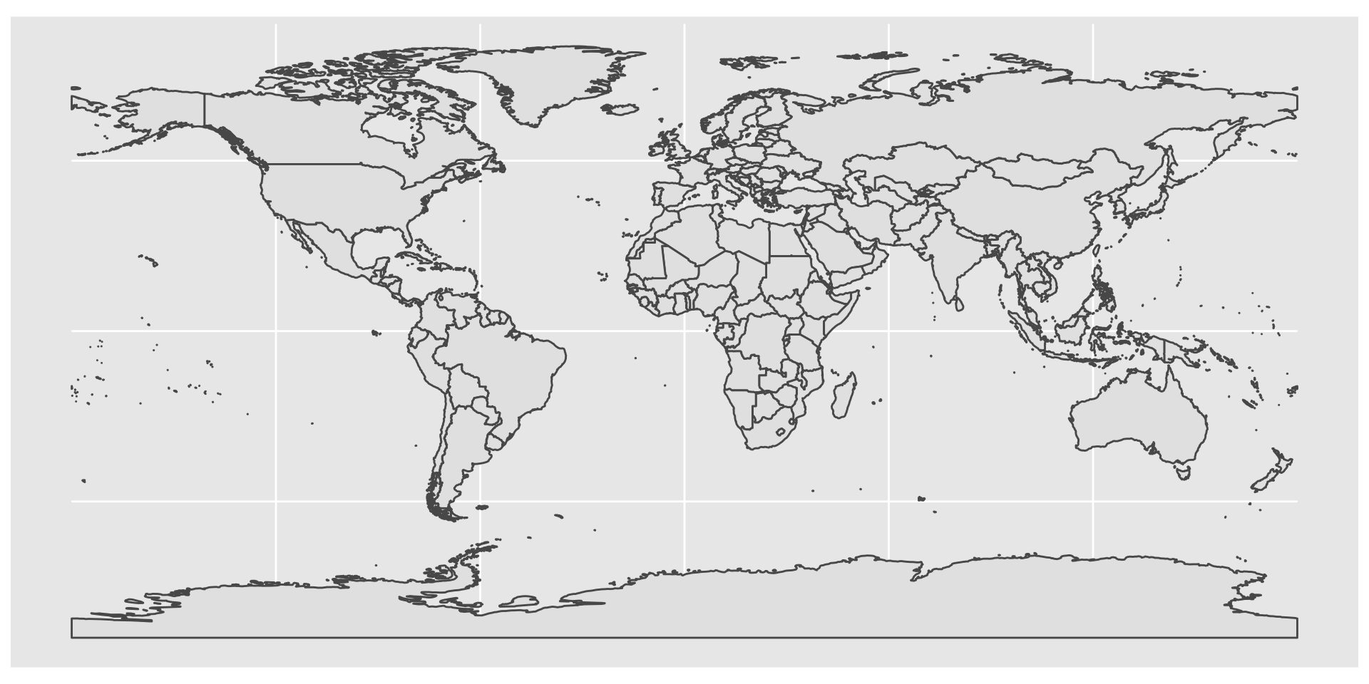
We now have data that we can plot by creating a base map of the world using ggplot2 package and ggplot function as shown below.

ggplot(data = aoi) +
  geom_sf()

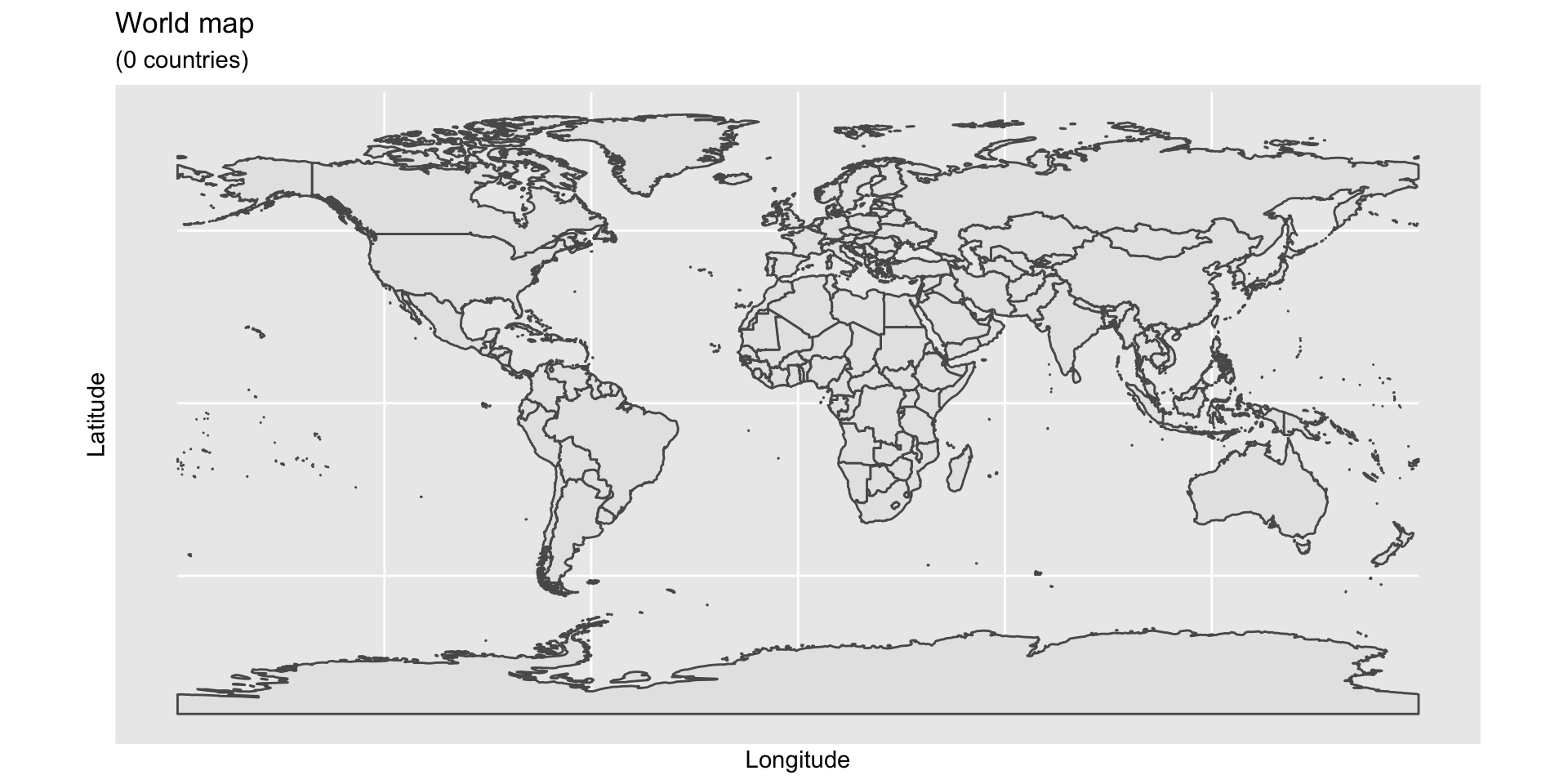
Further, we can add a title using ggtitle function, By default, Axis names are absent on a map, but can be changed to more suitable ones like “Longitude”….“Latitude”.

ggplot(data = aoi) +
  geom_sf() +
  xlab("Longitude") + ylab("Latitude") +
  ggtitle("World map", subtitle = paste0("(", length(unique(aoi$NAME)), " countries)"))

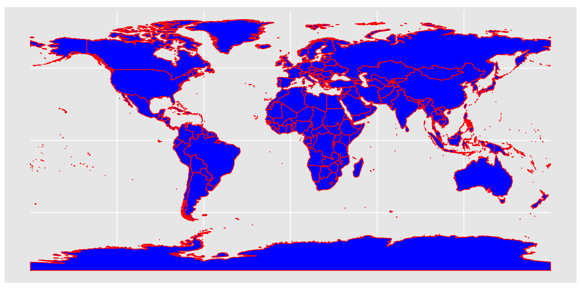
We now add some color by filling the polygons of the countries with a color, using argument fill and red for the outline of the countries using argument color.

ggplot(data = aoi) + 
  geom_sf(color = "red", fill = "blue")

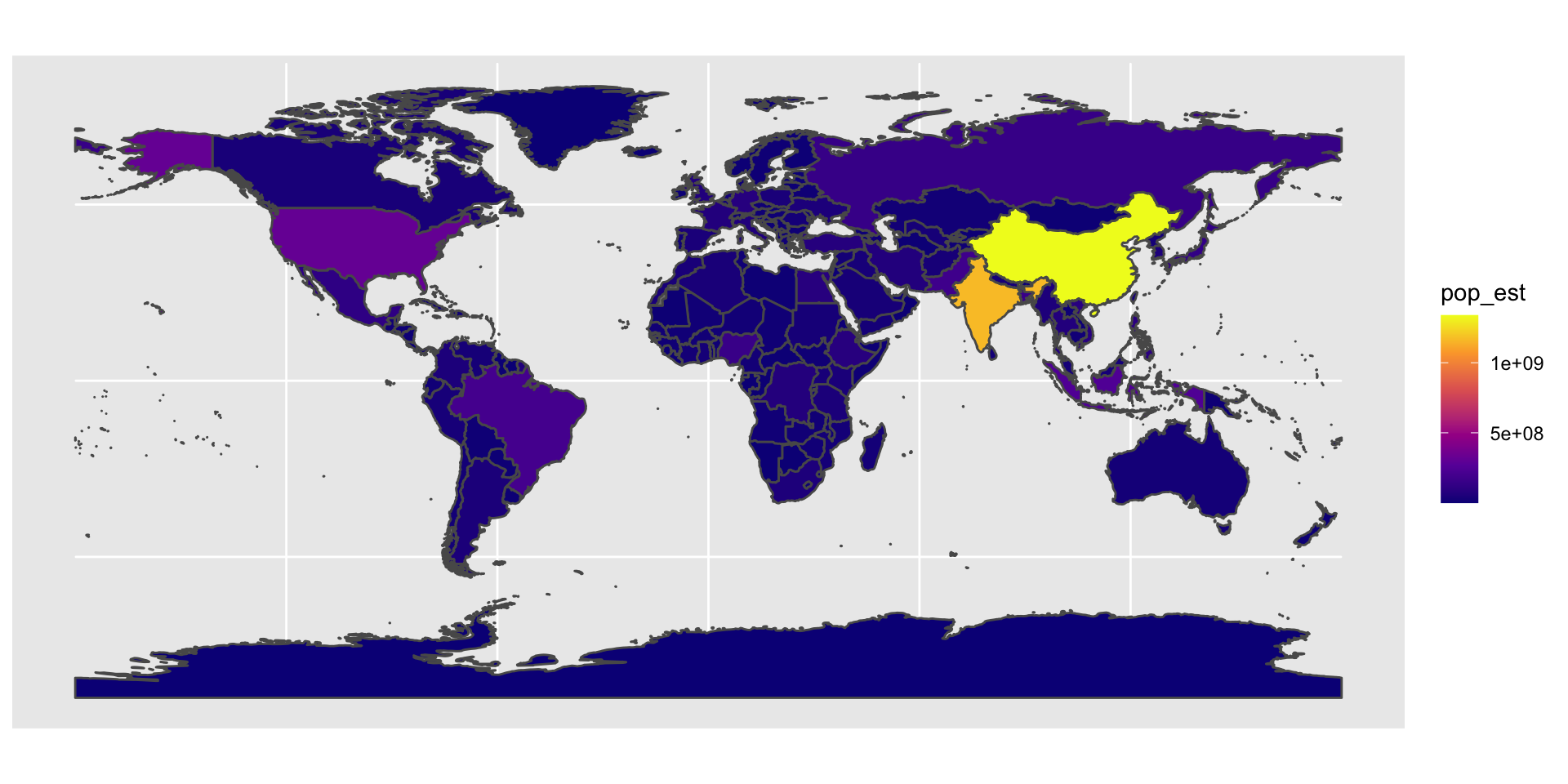
Visualization can get more interesting when you can show a gradient on one variable of the data - here we show the population of each country using the viridis scale through the option = "plasma".

ggplot(data = aoi) +
    geom_sf(aes(fill = pop_est)) +
    scale_fill_viridis_c(option = "plasma")

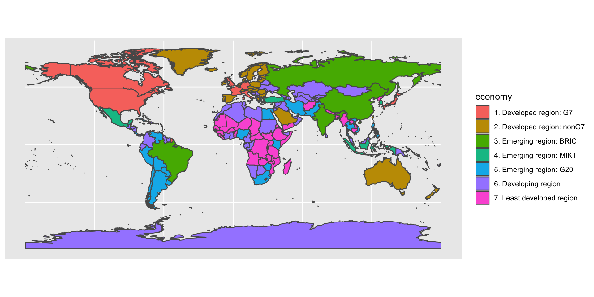
The object aoi contains various data that can be visualized. You can view what’s vailable through names(world). Here we visualize economies.

ggplot(data = aoi) +
    geom_sf(aes(fill = economy)) +
    scale_fill_discrete()

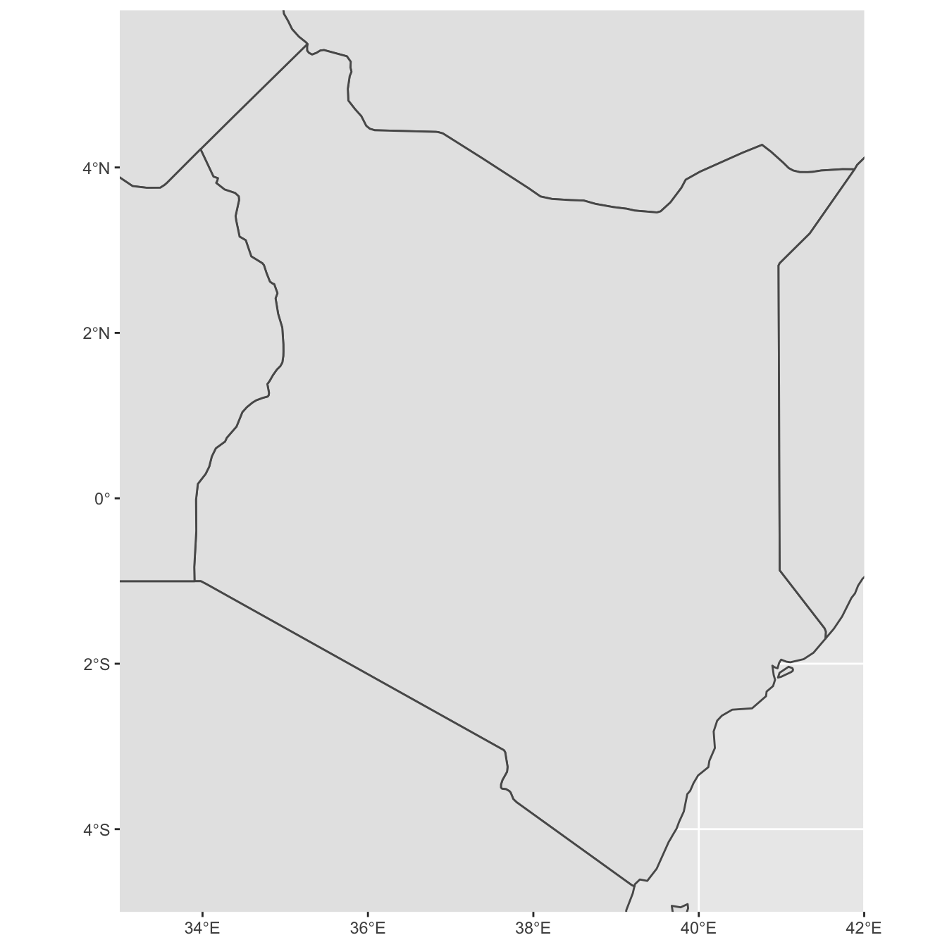
We can zoom in to any area of interest e.g Kenya, by setting the extent of the map using coord_sf function, and providing limits on the x-axis (xlim), and on the y-axis (ylim).

ggplot(data = aoi) +
    geom_sf() +
    coord_sf(xlim = c(33, 42), ylim = c(-5, 5.9), expand = FALSE)

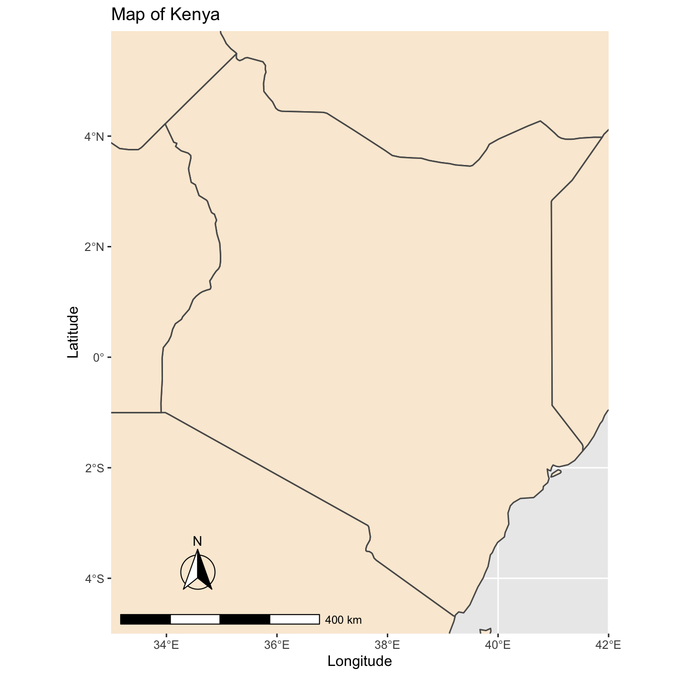
And add afew more elements to the map, but lets first load the ggspatial package through library(ggspatial). Check out these functions: annotation_scale, annotation_north_arrow and coord_sf and arguments: legend.position will automatically place the legend at a specific location, panel.grid.major and panel.grid.minor sets grid lines to gray color and have them appear dashed, panel.background colors the background. For more arguments see the function theme.

ggplot(data = aoi) +
  geom_sf(fill= "antiquewhite") +
  annotation_scale(location = "bl", width_hint = 0.45) +
  annotation_north_arrow(location = "bl", which_north = "true", 
                         pad_x = unit(0.6, "in"), pad_y = unit(0.4, "in"),
                         style = north_arrow_fancy_orienteering) +
  coord_sf(xlim = c(33, 42), ylim = c(-5, 5.9), expand = FALSE) +
  xlab("Longitude") + ylab("Latitude") +
  ggtitle("Map of Kenya")

Finally we save the map using ggsave function. Luckily, we have a choice of image formats to chose from e.g. PNG, JPEG, PDF etc Here we use PNG which is good for the web.

ggsave(paste0(iDir, "/"), "my_map.png", width = 6, height = 6, dpi = "screen")